1.  Introduction to the Instream Flow Reservation Process

The Instream Flow Reservation (IFR) application procedures requires the applicant to provide the hydrological, biological, and geographical data necessary to meet application standards. The reservation of instream flows is necessary for the production and maintenance of healthy anadromous and resident fish populations.

Templates and examples of all of this information is available in the IFR Notebook.

2.  The Site Selection Process

CE will fill in the prerequisites for site selection.

3.  Data Collection

1. An introductory note: Make sure that a clean copy of everything you copy or create is added to a "clean copy" folder. This will save you a lot of time later. Also, there are examples of all templates and files in the Folder. If anything is unclear, take a look there.

2. Create a folder in H:\common\Isf\Qstat\199Xresv\rivername to store the reservation files that you will be creating and filling out. Also label a folder for hard copies of output by rivername. You will also create a Brown folder.

3. Anadromous Waters Catalog (AWC): Print out Coor.xlt. The AWC and Atlas will allow you to do two things: first, determine the townships/ranges of the waterbody, and second, record the spawning, incubation, rearing, or passage information for each reach of the waterbody used by fish. Go to the AWC in Room A200 (or somewhere else if you are in SE) and look up the AWC number for the waterbody of interest. These are listed by region and are alphabetically in the back of the catalog. Copy down the number and USGS quad (i.e. 111-40-10010 Tyonek A-4). Now look at the large atlas for that region, starting from the quad number. Define all coordinates (Township, range, section) of the waterbody from the mouth to the origin by filling in Coor.xlt as you go. Include any sections in question. Coordinates will be recorded for each fish species as in p_krlk.xls. Anadromous species and life stage abbreviations are explained in the preface of the anadromous Catalog. Major anadromous tributaries are also noted and anadromous reach data is recorded for at least 2 sections above the confluence with the water body of concern. Make necessary edits and save as C_rivername.xls (c_krlk.xls) in the reservation folder.

4. Periodicity Data: The periodicity chart records which anadromous fishes utilize the waterbody at various life history stages. Periodicity charts are sent to ADF&G area biologists to complete. These are charts with all expected or known fish species in the waterbody. When returned they should be checked against the ADF&G sport fish harvest survey (reference 4). If there are discrepancies in fish species present, add the species in question. Hopefully the biologist has filled in period.xlt with the data – if not, copy periodicity data into the spreadsheet. When preparing the periodicity tables, make sure that there are only four species per page .. it will look odd now but when you transfer the tables to the reservation report it will save you a great deal of time. Also, make sure each species has its own table … "Dolly Varden/Arctic char" is not acceptable. Save as P_rivername.xls (p_krlk.xls) in the reservation folder.

Some points to remember:

• In the periodicity tables, spawning = incubation. If there is spawning occurring, make sure that incubation is occurring at the same time.

• Doublecheck that species in periodicity chart are the same as those in the reservation (5b).

• Put only four species on each page in period.xlt. This will make it much easier to copy them to the reservation (they won’t be too big to be inserted as objects into the word document). Instructions for pasting excel tables and charts into the reservation document is in Appendix 2.

• Species name should be in bold, and if it is a long name (such as "humpback whitefish") make the font smaller so it all fits on one line.

4.  Creating Reach and Area Maps

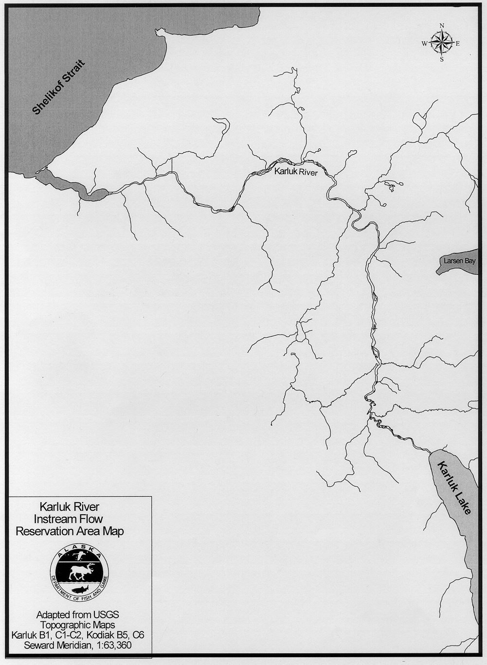
See ArcView Tutorial 3 for instructions on how to create instream flow maps; see examples below.

ISF Reach Map	ISF Area Map

5.  Data Analysis

A. IFR Data Analysis using SAS

USGS streamflow data are collected for each waterbody in which flows are to be reserved. There are several steps to follow when acquiring these data:

1. Look up waterbody in Alaska Index: Streamflow, Lake Levels, and Water-Quality Records to September 10, 1988. They are listed by gage number and alphabetically Copy the page with the gage information (make sure you get all pages and file in the reservation folder.

2. Reference the Internet and download all available data using the USGS site http://waterdata.usgs.gov/nwis-w/AK/. Fill in the gage number and click "Retrieve data". Click on "Historical Streamflow Daily Values". When the years of reference appear, note all record years for the gage. If there are multiple years of record, change the input fields to include all years and select "Tab delimited". Name files as site #.dta and save to the Qstat/19XX/rivername folder you created for the reservation. From this information you will see all years for which gage information is available.

3. Reference USGS document "Alaska Water Resource Data 19XX" for each waterbody. A hard copy of the last full year of record should be made and added to the reservation file folder. This information will tell you about the history of the gage; for instance, if there have been diversions, if the gage has been washed out, etc. Example in Appendix.

4.   Using the saved USGS streamflow data files, statistical analyses are conducted using SAS. Copy site#.dta to H:\BIO\CE_AEB\. Open site#.dta file (use notepad), and look for errors (e.g. deleting any lines) Within the same directory (H:\ BIO\CE_AEB\) find the shortcut file called if1998.sas (it is 1KB and is the SAS System Program, icon at right) which is an automated SAS program. Edit the file with right click, send to, notepad, and follow the instructions on the first page. Look at Appendix XXX for an example of this document. Remember that you have to save every time!!!!! If you don’t have Notepad in your send to menu, look in the Resources section to create the icon.

5.   Double click the if1998.lnk shortcut (see at right). SAS then creates output within a newly created sub-directory with the name of the site #, including automatically outputted graphs. Make sure you make copies of these graphs and store a clean copy.

6. Open the gagenumber.log file within this directory with the right click, send to, notepad, and search for errors or warnings using the find command (control-f). If errors are found, document them and send the list and the log file as attachment to Allen Bingham by email.

7. Now open the Word documents in this folder. In Explorer, you can select all of them and hit "enter" to open all of them at once. You will format them with the "format word macro" Ctrl-Alt-I. Instructions for creating this macro can be found in Appendix XXX. This macro deletes the first blank page, changes font to courier new, and font to size 7. These files are saved in doc/text format and need to be changed to native *.doc;  follow these instructions for each document: F12, Tab, up arrow 3X, Enter, Enter. This opens the "save as" dialog box, tabs to the "file type" box, goes up to "*.doc" format, and saves. Do this for each document and print them out. Make a copy, putting one in the brown folder and one in a clean copy folder.

8. Graphs can be reprinted two ways, although I am currently trying to find a better way. 1). With the replot.sas file; see Appendix XXX. 2). From the *.cgm files in the gagenumber folder, if necessary. See Appendix XXX for instructions on this process. These graphs are nice to add to the final report.

B. Tennant Analysis

Using data from the SAS output and provided by CE, you will now fill in the T_10rvr.xlt spreadsheet. You can do this one on the computer. When you open it you will note that several of the cells on the first two sheets have red triangles in the upper right corners. Hold the cursor over these and they will tell you what information to input into the cells. This will automatically build the charts on sheets three and four. The "Instream Flow Requirements" data on the second sheet will come from Christopher when he conducts his analysis. The only other thing you need to do is add a title to the charts and make sure that the axes are formatted as per the examples in the appendices.  Save the file as 10_karluk.xls.

 

6.  Reservation Form

T_reserv.doc is the Reservation Application Form. This form has instructions on it, so just follow them. Highlighted areas need to be replaced with the proper information. Note: it is vital to check your input to this document well. Using search and replace is convenient but problematic at times. Make sure that all numbers, names, values, etc are correct. Example in Appendix. For periodicity, only 4 per page. Appendix XXX for info on pasting periodicity and other info. You’ll need ArcView Reach and Area Maps and the replotted SAS data to import the hydrograph into the report.

7.  Master Folder

A master folder will be created containing ..xxx x xx x x x x

8.  Year-end Report

The yearly report is a compilation of the current year reservations. A template called yr_rept.doc can be found in the templates directory. You will need copies of the tables, graphs, and maps from the individual reservations (copied from the word document) as well as updated reservation location maps for that year and 1986-19xx. These maps are in the ArcView directories. The species list is a summary of all species found in that year’s periodicity tables. Summary of USGS gages. Tennant tables for each. Historical data summary of USGS gages in AK.

9.  ISF Appendix Table of Contents:

Appendix 1: ISF Data and Info
Appendix 2: Pasting Tables and Graphs into the Reports
Appendix 3: Editing the IF1998.sas Program
Appendix 4: Example of a USGS *.dta File
Appendix 5: SAS Output Guide
Appendix 6: How to use the SAS replot module
Appendix 7: Fish Species List
Appendix 8: How to Make a Word Macro